Note
Go to the end to download the full example code.
Morlet Wavelet spectrogram plot
Below is a code sample for plotting wavelet spectrograms
from pyqtgraph.examples.ViewBox import yScale

from ieeg.viz.ensemble import chan_grid
from bids import BIDSLayout
from ieeg.navigate import channel_outlier_marker, trial_ieeg, outliers_to_nan
from ieeg.io import raw_from_layout
from ieeg.calc.scaling import rescale
from ieeg.timefreq.utils import crop_pad
from ieeg.timefreq.superlets import superlet_tfr, superlets
from ieeg.viz.parula import parula_map
import numpy as np
import mne
import matplotlib.pyplot as plt
from matplotlib.gridspec import GridSpec
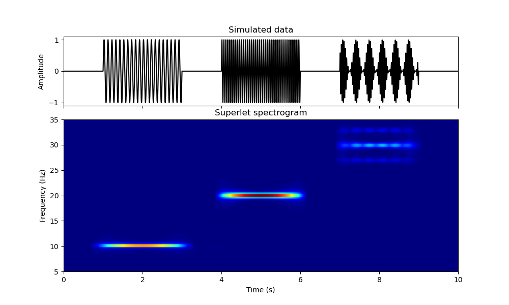
Simulate a 1D signal with some bursts of 10, 20, and 70 Hz and a sampling rate of 1000 Hz
fs = 1000
frange = (5, 35)
trange = (0, 10)
t = np.arange(trange[0], trange[1], 1 / fs)
burst = np.sin(2 * np.pi * 3 * t) + 1
s1 = np.sin(2 * np.pi * 10 * t) * (t > 1) * (t < 3)
s2 = np.sin(2 * np.pi * 20 * t) * (t > 4) * (t < 6)
s3 = np.sin(2 * np.pi * 30 * t) * (t > 7) * (t < 9) * burst / 2
data = s1 + s2 + s3
data = data[np.newaxis, :]

# run the superlet transform
freqs = np.linspace(frange[0], frange[1], 100)
wavelet = superlets(data, fs, freqs, 5, (10, 20))

# Create a figure and GridSpec layout
fig = plt.figure(figsize=(10, 6))
gs = GridSpec(3, 1, figure=fig)  # 3 rows: 1 for signal, 2 for spectrogram

# Add the signal plot (1/3 of the height)
ax_signal = fig.add_subplot(gs[0, 0])
ax_signal.plot(t, data[0], color='k')
ax_signal.set_title("Simulated data")
ax_signal.set_ylabel("Amplitude")

# Add the spectrogram plot (2/3 of the height)
ax_spectrogram = fig.add_subplot(gs[1:, 0], sharex=ax_signal)  # Spans the last 2 rows
ax_spectrogram.imshow(wavelet, aspect='auto', origin='lower',
                      extent=[trange[0], trange[1], frange[0], frange[1]],
                      cmap='jet')
ax_spectrogram.set_title("Superlet spectrogram")
ax_spectrogram.set_ylabel("Frequency (Hz)")
ax_spectrogram.set_xlabel("Time (s)")

# Hide x-axis labels for the top plot to avoid overlap
plt.setp(ax_signal.get_xticklabels(), visible=False)
[None, None, None, None, None, None]
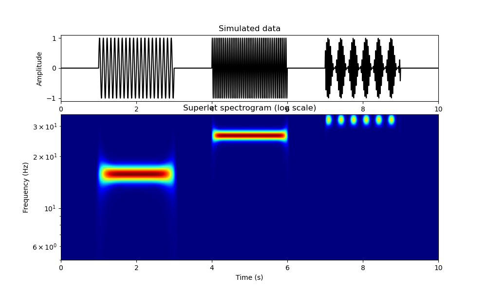
Do the transform again with log scaling
freqs = np.geomspace(frange[0], frange[1], 100)
wavelet = superlets(data, fs, freqs, 1.26, (10,10))

# Create a new figure and GridSpec layout
fig_log = plt.figure(figsize=(10, 6))
gs_log = GridSpec(3, 1, figure=fig_log)  # 3 rows: 1 for signal, 2 for spectrogram

# Add the signal plot (1/3 of the height)
ax_signal_log = fig_log.add_subplot(gs[0, 0])
ax_signal_log.plot(t, data[0], color='k')
ax_signal_log.set_title("Simulated data")
ax_signal_log.set_ylabel("Amplitude")

# Add the spectrogram plot (2/3 of the height)
ax_spectrogram_log = fig_log.add_subplot(gs[1:, 0], sharex=ax_signal_log)  # Spans the last 2 rows
ax_spectrogram_log.imshow(wavelet, aspect='auto', origin='lower',
                            extent=[trange[0], trange[1], freqs[0], freqs[-1]],
                            cmap='jet')
ax_spectrogram_log.set_yscale('log')
ax_spectrogram_log.set_title("Superlet spectrogram (log scale)")
ax_spectrogram_log.set_ylabel("Frequency (Hz)")
ax_spectrogram_log.set_xlabel("Time (s)")
Text(0.5, 36.72222222222221, 'Time (s)')
Load Data
bids_root = mne.datasets.epilepsy_ecog.data_path()
layout = BIDSLayout(bids_root)
filt = raw_from_layout(layout, subject="pt1", preload=True,
                      extension=".vhdr")
Extracting parameters from /home/docs/mne_data/MNE-epilepsy-ecog-data/sub-pt1/ses-presurgery/ieeg/sub-pt1_ses-presurgery_task-ictal_ieeg.vhdr...
Setting channel info structure...
Reading events from /home/docs/mne_data/MNE-epilepsy-ecog-data/sub-pt1/ses-presurgery/ieeg/sub-pt1_ses-presurgery_task-ictal_events.tsv.
Reading channel info from /home/docs/mne_data/MNE-epilepsy-ecog-data/sub-pt1/ses-presurgery/ieeg/sub-pt1_ses-presurgery_task-ictal_channels.tsv.
Reading electrode coords from /home/docs/mne_data/MNE-epilepsy-ecog-data/sub-pt1/ses-presurgery/ieeg/sub-pt1_ses-presurgery_space-fsaverage_electrodes.tsv.
/home/docs/checkouts/readthedocs.org/user_builds/ieeg-pipelines/checkouts/latest/ieeg/io.py:283: RuntimeWarning: DigMontage is only a subset of info. There are 3 channel positions not present in the DigMontage. The channels missing from the montage are:

['RQ1', 'RQ2', 'N/A'].

Consider using inst.rename_channels to match the montage nomenclature, or inst.set_channel_types if these are not EEG channels, or use the on_missing parameter if the channel positions are allowed to be unknown in your analyses.
  whole_raw = read_raw_bids(bids_path=BIDS_path, verbose=verbose)
/home/docs/checkouts/readthedocs.org/user_builds/ieeg-pipelines/checkouts/latest/ieeg/io.py:283: RuntimeWarning: Unable to map the following column(s) to to MNE:
outcome: S
engel_score: 1.0
ilae_score: 2.0
date_follow_up: n/a
ethnicity: 0.0
years_follow_up: 3.0
site: NIH
clinical_complexity: 1.0
  whole_raw = read_raw_bids(bids_path=BIDS_path, verbose=verbose)
Reading 0 ... 269079  =      0.000 ...   269.079 secs...
Crop raw data to minimize processing time
new = filt.copy()

# Mark channel outliers as bad
new.info['bads'] = channel_outlier_marker(new, 5)

# Exclude bad channels
good = new.copy().drop_channels(new.info['bads'])
good.load_data()

# Remove intermediates from mem
del new
outlier round 1 channels: ['N/A']
outlier round 2 channels: ['N/A', 'RQ2']
outlier round 3 channels: ['N/A', 'RQ2', 'AST2']
outlier round 4 channels: ['N/A', 'RQ2', 'AST2', 'AD3']
outlier round 5 channels: ['N/A', 'RQ2', 'AST2', 'AD3', 'PD4']
outlier round 6 channels: ['N/A', 'RQ2', 'AST2', 'AD3', 'PD4', 'G32']
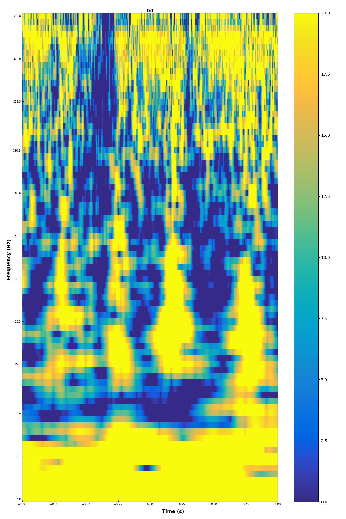
Calculate Spectra
for epoch, t in zip(
        ("onset", "offset"),
        ((-1, 0), (-1, 1)),):
    times = [None, None]
    times[0] = t[0] - 0.5
    times[1] = t[1] + 0.5
    trials = trial_ieeg(good, epoch, times, preload=True, picks=[0])
    outliers_to_nan(trials, outliers=10)
    freqs = np.geomspace(4, 500, 80)
    spec = superlet_tfr(trials, freqs, 1., (15, 15))
    crop_pad(spec, "0.5s")
    if epoch == "onset":
        base = spec.copy()
        continue
    spec_a = rescale(spec, base, copy=True, mode='logratio').average(
        lambda x: np.nanmean(x, axis=0), copy=True)
    spec_a._data = spec_a._data * 20
Used Annotations descriptions: [np.str_('AD1-4, ATT1,2'), np.str_('AST1,3'), np.str_('G16'), np.str_('PD'), np.str_('SLT1-3'), np.str_('offset'), np.str_('onset')]
Not setting metadata
1 matching events found
No baseline correction applied
0 projection items activated
Using data from preloaded Raw for 1 events and 2001 original time points ...
0 bad epochs dropped
[Parallel(n_jobs=1)]: Done   1 tasks      | elapsed:    0.1s
[Parallel(n_jobs=1)]: Done   1 out of   1 | elapsed:    0.1s finished
Used Annotations descriptions: [np.str_('AD1-4, ATT1,2'), np.str_('AST1,3'), np.str_('G16'), np.str_('PD'), np.str_('SLT1-3'), np.str_('offset'), np.str_('onset')]
Not setting metadata
1 matching events found
No baseline correction applied
0 projection items activated
Using data from preloaded Raw for 1 events and 3001 original time points ...
0 bad epochs dropped
[Parallel(n_jobs=1)]: Done   1 tasks      | elapsed:    0.2s
[Parallel(n_jobs=1)]: Done   1 out of   1 | elapsed:    0.2s finished
Applying baseline correction (mode: logratio)
Plot data
chan_grid(spec_a, vlim=(0, 20), cmap=parula_map, yscale='log', n_cols=1, n_rows=1)
No baseline correction applied

[<Figure size 1200x1800 with 2 Axes>]
Total running time of the script: (0 minutes 6.508 seconds)
Estimated memory usage: 1345 MB
Related examples